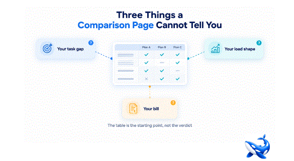
Three Things a Comparison Page Cannot Tell You

A model comparison table is where good decisions start, and it is also where they stall, because the page deliberately cannot answer three questions that every rollout has to answer anyway. On OrcaRouter‘s compare llm models page the limits are visible in the data itself, read 2026-10-12: eleven of the twelve rows sit between an 8.0 and a 10.0 on our composite quality score, while their input prices span fifty times, from $0.60 to $30.00. A page that compresses quality into a two-point band and stretches price across two orders of magnitude is telling you, in the clearest possible way, which of its columns you should treat as a floor and which you should treat as a decision.

The table narrows. The three blind spots below decide.

What the two-point quality band means for your task

The first thing the page cannot tell you is what the gap between an 8.0 and a 9.0 does to your specific workload. The composite quality score is our own judgment — we score each model ourselves across quality dimensions such as instruction adherence, reasoning quality, output coherence and consistency — so it is a defensible floor, but it is not a benchmark of your task. When eleven of twelve rows land inside a two-point band, the column is telling you that these models are close in general quality, not that they are interchangeable on your summarization pipeline or your retrieval loop.

Where the gap has to come from instead: your own task-level test. Take the two or three rows that clear your floor, run them on a sample of your real prompts, and grade the outputs against the cases that actually break in production. The page can tell you the models are close; only your traces can tell you whether that closeness holds on the one task you are paying for. This is not an argument against the table — it is an argument for using the table to build the test.

The same logic applies to the traffic column. Seven-day token volume is a wonderful signal about the market — it tells you which rows real workloads lean on, and that is exactly the information a lone benchmark score hides. But it answers the question “where is the crowd?” rather than “where should we go?” A row carrying 512.0M tokens is popular for a reason, and a row carrying 101.8K is niche for a reason, and neither reason transfers to your task unchanged. Treat the volume column as a popularity read, not as a recommendation.

The shape of latency under your own load

The second thing the page cannot tell you is the distribution behind a single latency number. A p50 time to first token is one honest figure, and the page is careful with it — the caveats matter. Eleven of the twelve rows show a ninety-fifth-percentile reading sitting exactly at the 10.00 s ceiling, which is the measurement ceiling, not a measured spread, and several rows show a p50 of exactly 10.00 s, the same ceiling. What the page cannot render is how those numbers behave when twenty requests arrive at once, or when your prompts are long, or when the model is serving its whole vendor region at peak.

That last condition is the one nobody can pre-compute for you. The measurement ceiling is not a design flaw; it is a boundary the page draws honestly between what it could capture and what it could not. But a boundary is exactly the place where a rollout plan needs its own instrumentation. Two models with identical medians can feel completely different to a user, because the tail — the requests that take twice as long, or fail outright — is what humans actually notice. Medians describe the comfortable middle; the tail describes the experience.

Where the shape has to come from instead: a load test in staging. Run your own concurrency, your own prompt sizes, your own timeout budget, and read the distribution, not the median. A p50 of 3.29 s with a tail at the ceiling tells you the middle is comfortable and the tail is unknown; the only way to learn what the tail does to your users is to generate a tail with your own traffic.

The bill for your mix, not the price for a token

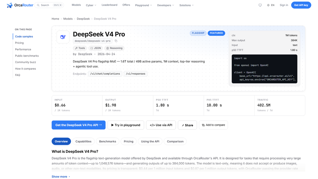
The third thing the page cannot tell you is your total bill, because cost is a function of your mix and your mix is nobody else’s. Input price alone misleads: DeepSeek V4 Pro charges $0.66 per million input tokens against $1.98 for output, a 3.0x output multiplier, while Gemini 3.1 Pro Preview charges $2.00 against $12.00, a 6.0x multiplier. On a read-heavy workload the cheap input row wins by a mile; on a write-heavy workload the multiplier reshuffles the ranking entirely. The page prints the four rates and the multiplier — it cannot print your read-to-write ratio.

Where the bill has to come from instead: a spreadsheet with your own volume. Estimate your monthly input tokens and output tokens, apply each row’s four numbers, and rank the result. The cheapest row on a per-token basis is not automatically the cheapest row on your workload, and the premium row is sometimes closer than the sticker shock suggests. Nobody else can run that arithmetic for you, because only you know what your prompts and your outputs actually look like.

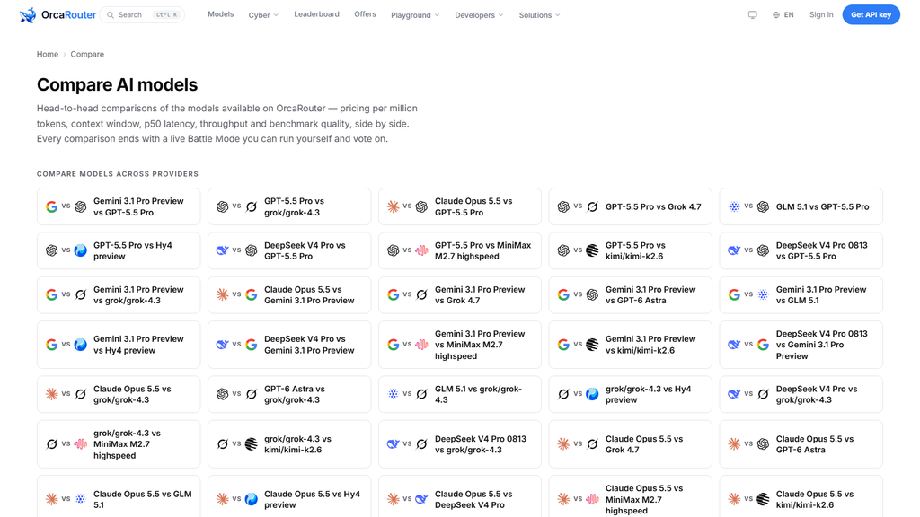
Where the page is deliberately thin

These three blind spots are not oversights. A comparison page that tried to carry your task test, your load shape and your bill would stop being a comparison page and become your internal documentation — which is where those three belong. The correct division of labor is that the page answers the questions that are true for everyone, read on a fixed date, and your rollout answers the questions that are true for you, re-run continuously. Trying to squeeze the second set out of the first is how teams end up arguing about tenths of a quality point that the page never claimed to measure.

That discipline shows up in the page’s own conventions. The latency and traffic figures are a rolling window and drift, which is why the read date travels with every number; the composite quality column is labelled as our own judgment, not a third-party benchmark; and the tail values that sit at the measurement ceiling are presented as a ceiling rather than as a measured spread. Every one of those conventions is the page telling you where its authority ends. The table is a snapshot of the field on one day — a good snapshot, but a snapshot.

The takeaway

A comparison page answers the questions that hold for everyone: prices, context windows, measured latency, our own composite quality judgment, and a snapshot of where the traffic went — all read 2026-10-12 and all rolling. What it cannot answer are the three questions that only your workload can settle: what a two-point quality gap does to your task, what the latency distribution does under your load, and what the price card does to your actual bill. Each one has to come from somewhere else: your task test, your staging load run, your own budget arithmetic.

The page is not the verdict; it is the evidence. Treat the quality column as the floor it honestly is, treat the price and latency columns as the decision they honestly are, and treat the three blind spots as your responsibility rather than the page’s failure. That is how a table becomes a shortlist.

Sourcing note: 所有数字 read 2026-10-12。Prices, context windows, latency readings and seven-day token volumes come from the OrcaRouter comparison page and the linked model page; the composite quality scores are our own, assigned across quality dimensions; ninety-fifth-percentile values sitting at the 10.00 s mark are the measurement ceiling, and p50 values of exactly 10.00 s are that same ceiling. Latency and volume figures are rolling windows and drift. All checked 2026-10-12.